Entropy/IP: Sample Report (Client IPv6 Addresses)

Entropy vs. 4-bit Aggregate Count Ratio (ACR)

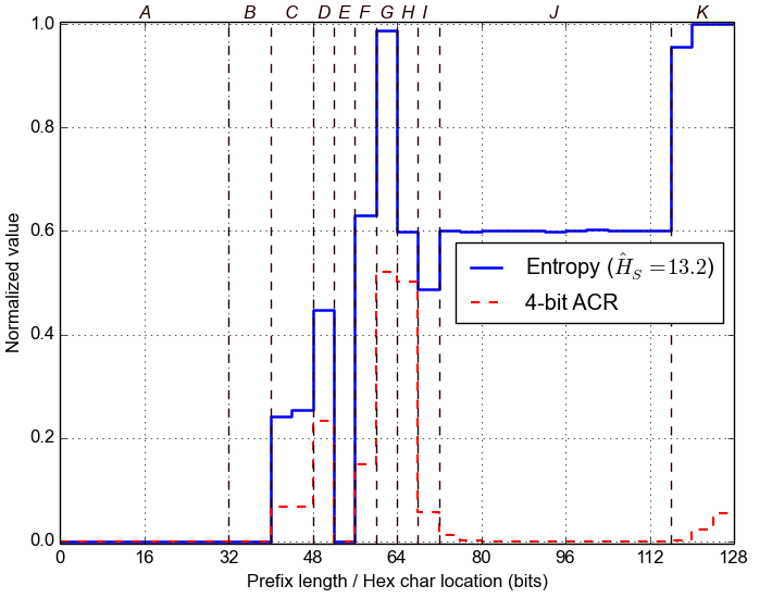
First, we estimate the Entropy for each nybble in the IPv6 addresses, across the whole dataset. For example, if the last nybble is highly variable, then the corresponding Entropy will be high. Conversely, the Entropy will be zero for nybbles that stay constant across the dataset. Below we plot the normalized value of Entropy for each of the 32 nybbles, along with the 4-bit Aggregate Count Ratio, which was introduced in Plonka and Berger, 2015.

Second, we group adjacent nybbles with similar Entropy to form larger segments, with the expectation that they represent semantically different parts of each address. We label these segments with letters and mark them with dashed lines in the plot below.

Segment Mining

Next, we search the segments for the most popular values and ranges of values within them. For that purpose, we use statistical methods for detecting outliers and the DBSCAN machine learning algorithm. We analyze distribution and frequencies of values inside address segments.

Below we present the results, with ranges of values shown as two values in italics (bottom to top). The last column gives the relative frequency across the whole dataset. The /32 prefixes are anonymized.

A: bits 0-32 (hex chars  1- 8)  20010db8                           100.00%
B: bits 32-40 (hex chars  9-10)  00                                 100.00%
C: bits 40-48 (hex chars 11-12)  10                                  60.59%
  22                                  37.86%
  20                                   0.82%
  21                                   0.74%
D: bits 48-52 (hex chars 13-13)  0                                   59.62%
  1                                   13.85%
  3                                   12.29%
  2                                    7.12%
  4                                    6.56%
  5                                    0.26%
  7                                    0.14%
  d                                    0.11%
E: bits 52-56 (hex chars 14-14)  0                                  100.00%
F: bits 56-60 (hex chars 15-15)  0                                   49.99%
  1                                   18.51%
  6                                    5.27%
  2                                    3.97%
  5                                    3.93%
* 3-d                                 18.33%
G: bits 60-64 (hex chars 16-16)  3                                    9.50%
  5                                    7.87%
  4                                    7.63%
  8                                    7.48%
* 0-f                                 67.52%
H: bits 64-68 (hex chars 17-17)  0                                   63.06%
  1                                    2.62%
  d                                    2.55%
  9                                    2.55%
  5                                    2.55%
* 2-f                                 26.67%
I: bits 68-72 (hex chars 18-18)  0                                   65.13%
  8                                    5.11%
  1                                    5.06%
  5                                    4.95%
  9                                    4.90%
* 2-f                                 14.84%
J: bits 72-116 (hex chars 19-29)  00000000000                         60.36%
* 0000ed18068-fffb2bc655b             39.64%
K: bits 116-128 (hex chars 30-32)  0ac                                  0.11%
  03a                                  0.11%
  089                                  0.10%
  02d                                  0.10%
  024                                  0.10%
  081                                  0.10%
  074                                  0.10%
  06e                                  0.10%
  06b                                  0.10%
  042                                  0.10%
* 000-fff                             99.00%

Bayesian Network Structure

Next, we search for statistical dependencies between the segments. For that purpose, we train a Bayesian Network (BN) from data.

Below we show structure of the corresponding BN model. Arrows indicate direct statistical influence. Note that directly connected segments can probabilistically influence each other in both directions (upstream / downstream). Under some conditions, segments without direct connection can still influence each other through other segments: e.g., A can influence C through B if C depends on B and B depends on A (even if there is no direct arrow between A and C).

Learning BN structure from data is in general a challenging optimization problem. Hence, there might be more than one possible BN structure graph for the same dataset.

Conditional Probability Browser

Finally, below we show an interactive browser that decomposes IPv6 addresses into segments, values, ranges, and their corresponding probabilities. The browser lets for exploring the underlying BN model and see how certain segment values probabilistically influence the other segments.

Try clicking on the colored boxes below. You should see the colors changing, which reflects the fact that some segment values can make the other values more (or less) likely. For instance, in the Sample Report, you may find that clicking on J1 (i.e., the first value in segment J) makes segments C, D, F, H, and I largely predictable (see our paper for more examples).

You may condition the model on many segment values. Clicking on selected values un-selects them. Clicking on the red "Clear" above the color map un-selects them all. Below the browser we show the estimated proportion of the addresses matching your selection (vs. the dataset). If the browser cannot estimate the probabilities in a reasonable time, it asks before trying harder.

Candidate Target Addresses

Using the BN model, below we generate a few candidate target IPv6 addresses matching the selection above. Note that we anonymize the IPv6 addresses in this report.

As we show in the paper, this technique allowed us to successfully scan IPv6 networks of servers and routers, and to predict the IPv6 network identifiers of active client IPv6 addresses.